What is Machine Learning?
A computer’s ability to learn from data without explicit programming is called machine learning.

It works like this: The machine learns from the existing data and predicts or makes decisions about future data. Your data set must contain known outcomes so that the machine can learn, take the data and adjust it, and apply the machine learning algorithm. The algorithm learns, creates a model, analyzes the model, and then uses that model to make predictions.
There are three main categories of machine learning algorithms:
- Supervised learning algorithms
- Unsupervised learning algorithms
- Reinforcement learning
Supervised Learning
Supervised learning refers to a data set with known outcomes. If it is unsupervised, there are no known outcomes and you won’t have the categories or classes necessary for the machine to learn.
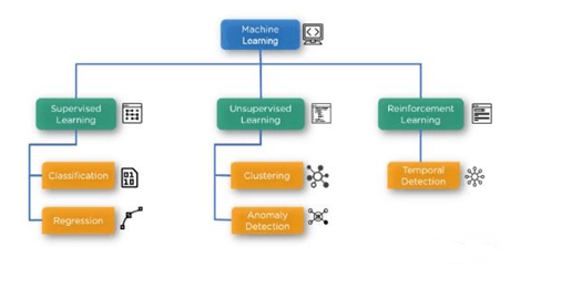
There are two major types of machine learning algorithms in the supervised learning category:
- Classification (which is covered under SVM)
- Regression
Classification Algorithms
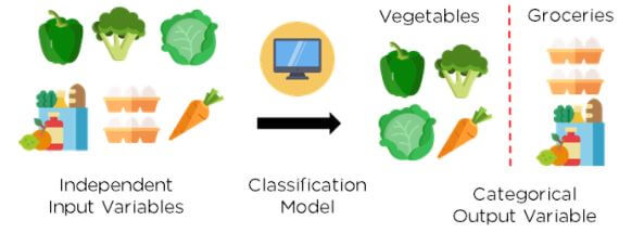
With classification, you predict categories while in regression, and you generally predict values.
In supervised learning, classification is multi-dimensional in the sense that sometimes you only have two classes (“yes” or “no”, or, “true” or “false”). But, sometimes you have more than two. For instance, under risk management or risk modeling, you can have “low risk”, “medium risk”, or “high risk.” SVM is a binary classifier (a classifier used for those true/false, yes/no types of classification problems).
Features are important in supervised learning. If there are several features, SVM may be the better classification algorithm choice as opposed to logistic regression. Under supervised learning, you present the computer with example inputs and their desired outputs (those known outcomes). The goal is to learn a general rule that maps inputs to those outputs.
Bug detection, customer churn, stock price prediction (not the value of the stock price, but whether or not it
will rise or fall), and weather prediction (sunny/not sunny; rain/no rain) are all examples.
Classification algorithms generally take past data (data for which you have known outcomes), train the model, take new data once the model is trained, ingest it, and create predictions (e.g., is it a truck or is it a car?).
What is SVM?
SVM is a type of classification algorithm that classifies data based on its features. An SVM will classify any new element into one of the two classes.
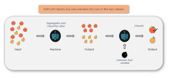
Once you give it some inputs, the algorithm will segregate and classify the data and then create the outputs. When you ingest more new data (an unknown fruit variable in this example), the algorithm will correctly classify the fruit: e.g., “apple” versus “orange”.
Example 1: Linear SVM classification problem with a 2D data set
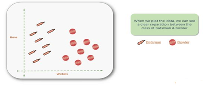
The goal of this example is to classify cricket players into batsmen or bowlers using the runs-to-wicket ratio. A player with more runs would be considered a batsman and a player with more wickets would be considered a bowler.
If you take a data set of cricket players with runs and wickets in columns next to their names, you could create a two-dimensional plot showing a clear separation between bowlers and batsmen. Here we present a data set with clear segregation between bowlers versus batsmen to help understand SVM.
Before separating anything using high-level mathematics, let’s look at an unknown value, which is new data being introduced into the dataset without a predesignated classification.
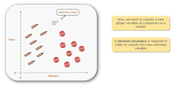
The next step is to draw a decision boundary, or a line separating the two classes to help classify the new data points.
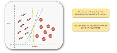
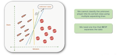
You can actually draw several boundaries, as shown above. Then, you need to find the line of best fit that clearly separates those two groups. The correct line will help you classify the new data point.
You can find the best line by computing the maximum margin from equidistant support vectors. Support vectors in this context simply mean the two points — one from each class that are closest together, but that maximize the distance between them or the margin.
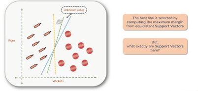
Note: You may think that the word vector refers to data points. While this may be the case in two-dimensional or three-dimensional spaces, once you get into higher dimensions with more features in your data set, you need to look at these as vectors. The reason they are support vectors is that the two vectors closest together maximize the distance between the two groups supporting the algorithm.
There are a couple of points at the top that are pretty close to one another, and similarly at the bottom of the graph. Shown below are the points that you need to consider. The rest of the points are too far away. The bowler points to the right and the batsman points to the left.
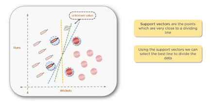
Mathematically, you can calculate the distance among all of these points and minimize that distance. Once you pick the support vectors, draw a dividing line, and then measure the distance from each support vector to the line. The best line will always have the greatest margin or distance between the support vectors.
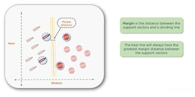
For instance, if you consider the yellow line as a decision boundary, the player with the new data point is the bowler. But, as the margins don’t appear to be maximum, you can come up with a better line.

Use other support vectors, draw the decision boundary between those, and then calculate the margin. Notice now that the unknown data point would be considered a batsman.
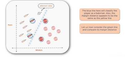
Continue doing this until you find the correct decision boundary with the greatest margin.
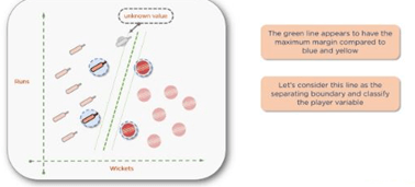
If you look at the green decision boundary, the line appears to have a maximum margin compared to the other two. This the boundary of greatest margin and when you classify your unknown data value, you can see that it clearly belongs to the batsman’s class. The green line divides the data perfectly because it has the maximum margin between the support vectors. At this point, you can be confident with the classification — the new data point is indeed a batsman.
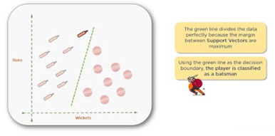
Technically, this dividing line is called a hyperplane. In two-dimensional spaces, we typically refer to the dividing lines as “lines,” but in three-dimensional and higher dimensions, they’re considered “planes” or “hyperplanes”. Technically, they are all hyperplanes.
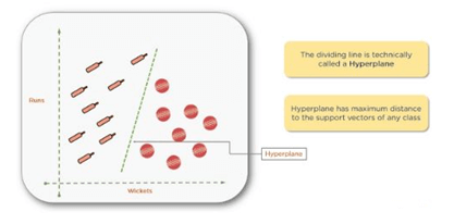
The hyperplane with the maximum distance from the support vectors is the one you want. Sometimes called the positive hyperplane (D+), it is the shortest distance to the closest positive point and (D-), or the negative hyperplane, which is the shortest distance to the closest negative point.

The sum of (D+) and (D-) is called the distance margin. You should always try to maximize the distance margin to avoid misclassification. For instance, you can see the yellow margin is much smaller than the green margin.

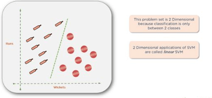
This problem set is two-dimensional because the classification is only between two classes. It is called a linear SVM.
Conclusion
SVM are based on statistical learning theory. They can be used for learning to predict future data. SVM are trained by solving a constrained quadratic optimization problem. SVM, implements mapping of inputs onto a high dimensional space using a set of nonlinear basis functions. SVM can be used to learn a variety of representations, such as neural nets, splines, polynomial estimators, etc, but there is a unique optimal solution for each choice of the SVM parameters. This is different in other learning machines, such as standard Neural Networks trained using back propagation.In short the development of SVM is an entirely different from normal algorithms used for learning and SVM provides a new insight into this learning. The four most major features of SVM are duality, kernels, convexity and sparseness.
Thank You
Mahendran M
Helical IT Solutions

Best Open Source Business Intelligence Software Helical Insight is Here
